The Relational Data Model, Normalisation and effective Database Design

Introduction

What is a database?

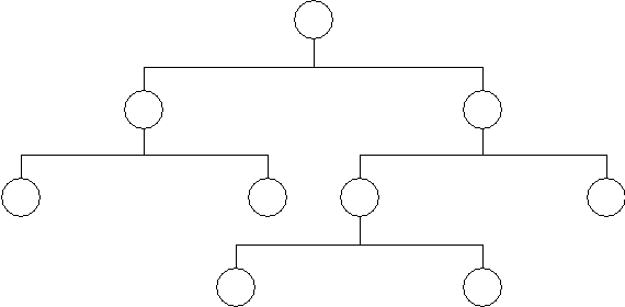
The Hierarchical Data Model

The Network Data Model

The Relational Data Model

The Relation

Keys

Compound Keys with NULL values

Relationships

Referential Integrity

Relational Joins

Lossless Joins

Determinant and Dependent

Functional Dependencies (FD)

Transitive Dependencies (TD)

Multi-Valued Dependencies (MVD)

Join Dependencies (JD)

Modification Anomalies

Types of Relational Join

Inner Join

Natural Join

Left [Outer] Join

Right [Outer] Join

Full [Outer] Join

Self Join

Cross Join

Entity Relationship Diagram (ERD)

Data Normalisation

1st Normal Form

2nd Normal Form

3rd Normal Form

Boyce-Codd Normal Form

4th Normal Form

5th (Projection-Join) Normal Form

6th (Domain-Key) Normal Form

De-Normalisation

Compound Fields

Summary Fields

Summary Tables

Optional Attributes that exist as a group

Personal Guidelines

Database Names

Table Names

Field Names

Primary Keys

Foreign Keys

Generating Unique ids

Criticisms

The choice between upper and lower case

The use of unique and non-unique field names

Field names should identify their content

The naming of Foreign Keys

References

Amendment History

Comments

Introduction

I have been designing and building applications, including the databases used by those applications, for several decades now. I have seen similar problems approached by different designs, and this has given me the opportunity to evaluate the effectiveness of one design over another in providing solutions to those problems.

It may not seem obvious to a lot of people, but the design of the database is the heart of any system. If the design is wrong then the whole application will be wrong, either in effectiveness or performance, or even both. No amount of clever coding can compensate for a bad database design. Sometimes when building an application I may encounter a problem which can only be solved effectively by changing the database rather than by changing the code, so change the database is what I do. I may have to try several different designs before I find one that provides the most benefits and the least number of disadvantages, but that is what prototyping is all about.

The biggest problem I have encountered in all these years is where the database design and software development are handled by different teams. The database designers build something according to their rules, and they then expect the developers to write code around this design. This approach is often fraught with disaster as the database designers often have little or no development experience, so they have little or no understanding of how the development language can use that design to achieve the expected results. This happened on a project I worked on in the 1990s, and every time that we, the developers, hit a problem the response from the database designers was always the same: Our design is perfect, so you will have to just code around it. So code around it we did, and not only were we not happy with the result, neither were the users as the entire system ran like a pig with a wooden leg.

In this article I will provide you with some tips on how I go about designing a database in the hope that you may learn from my experience. Note that I do not use any expensive modelling tools, just the Mark I Brain.

What is a database?

This may seem a pretty fundamental question, but unless you know what a database consists of you may find it difficult to build one that can be used effectively. Here is a simple definition of a database:

A database is a collection of information that is organised so that it can easily be accessed, managed, and updated.

A database engine may comply with a combination of any of the following:

• The database is a collection of table, files or datasets.
• Each table is a collection of fields, columns or data items.
• One or more columns in each table may be selected as the primary key.
• There may be additional unique keys or non-unique indexes to assist in data retrieval.
• Columns may be fixed length or variable length.
• Records may be fixed length or variable length.
• Table and column names may be restricted in length (8, 16 or 32 characters).
• Table and column names may be case-sensitive.

Over the years there have been several different ways of constructing databases, amongst which have been the following:

• The Hierarchical Data Model
• The Network Data Model
• The Relational Data Model

Although I will give a brief summary of the first two, the bulk of this document is concerned with The Relational Data Model as it the most prevalent in today's world. Other types of database model are described here.

The Hierarchical Data Model

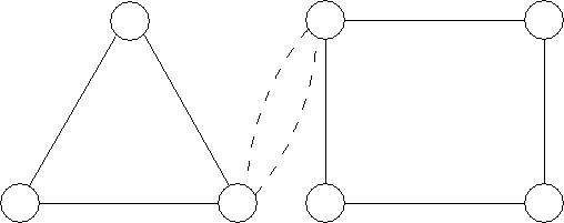
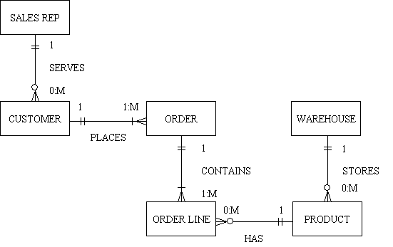
The Hierarchical Data Model structures data in a tree of records, with each record having one parent record and many children. It can be represented as follows:

Figure 1 - The Hierarchical Data Model

A hierarchical database consists of the following:

1. It contains nodes connected by branches.
2. The top node is called the root.
3. If multiple nodes appear at the top level, the nodes are called root segments.
4. The parent of node n^x is a node directly above n^x and connected to n^x by a branch.
5. Each node (with the exception of the root) has exactly one parent.
6. The child of node n^x is the node directly below n^x and connected to n^x by a branch.
7. One parent may have many children.

By introducing data redundancy, complex network structures can also be represented as hierarchical databases. This redundancy is eliminated in physical implementation by including a 'logical child'. The logical child contains no data but uses a set of pointers to direct the database management system to the physical child in which the data is actually stored. Associated with a logical child are a physical parent and a logical parent. The logical parent provides an alternative (and possibly more efficient) path to retrieve logical child information.

The Network Data Model

The Network Data Model uses a lattice structure in which a record can have many parents as well as many children. It can be represented as follows:

Figure 2 - The Network Data Model

Like the The Hierarchical Data Model, the Network Data Model also consists of nodes and branches, but a child may have multiple parents within the network structure instead of being restricted to just one.

I have worked with both hierarchical and network databases, and they both suffered from the following deficiencies (when compared with relational databases):

• Access to the database was not via SQL query strings, but by a specific set of API's, typically for FIND, CREATE, READ, UPDATE and DELETE.
• Each API would only access a single table (dataset), so it was not possible to implement a JOIN which would return data from several tables.
• It was not possible to provide a variable WHERE clause. The only selection mechanism available was
  • read all entries (a full table scan).
  • read a single entry using a specific primary key.
  • read all entries on a child table which were associated with a selected entry on a parent table
  Any further filtering had to be done within the application code.
• It was not possible to provide an ORDER BY clause. Data was presented in the order in which it existed in the database. This mechanism could be tuned by specifying sort criteria to be used when each record was inserted, but this had several disadvantages:
  • Only a single sort sequence could be defined for each path (link to a parent), so all records retrieved on that path would be provided in that sequence.
  • It could make inserts rather slow when attempting to insert into the middle of a large collection, or where a table had multiple paths each with its own set of sort criteria.
• It was not possible for the database to maintain Referential Integrity between parent and child tables. This had to be done entirely with application code.

The Relational Data Model

The Relational Data Model has the relation at its heart, but then a whole series of rules governing keys, relationships, joins, functional dependencies, transitive dependencies, multi-valued dependencies, and modification anomalies.

The Relation

The Relation is the basic element in a relational data model.

Figure 3 - Relations in the Relational Data Model

A relation is subject to the following rules:

1. Relation (file, table) is a two-dimensional table.
2. Attribute (i.e. field or data item) is a column in the table.
3. Each column in the table has a unique name within that table.
4. Each column is homogeneous. Thus the entries in any column are all of the same type (e.g. age, name, employee-number, etc).
5. Each column has a domain, the set of possible values that can appear in that column.
6. A Tuple (i.e. record or occurrence) is a row in the table.
7. The order of the rows and columns is not important.
8. Values of a row all relate to some thing or portion of a thing.
9. Repeating groups (collections of logically related attributes that occur multiple times within one record occurrence) are not allowed.
10. Duplicate rows are not allowed (candidate keys are designed to prevent this).
11. Cells must be single-valued (but can be variable length). Single valued means the following:
    • Cannot contain multiple values such as 'A1,B2,C3'.
    • Cannot contain combined values such as 'ABC-XYZ' where 'ABC' means one thing and 'XYZ' another.

A relation may be expressed using the notation R(A,B,C, ...) where:

• R = the name of the relation.
• (A,B,C, ...) = the attributes within the relation.
• A = the attribute(s) which form the primary key.

Keys

1. A simple key contains a single attribute.
2. A composite key (or compound key) is a key that contains more than one attribute.
3. A candidate key is an attribute (or set of attributes) that uniquely identifies a row. A candidate key must possess the following properties:
   • Unique identification - For every row the value of the key must uniquely identify that row.
   • Non redundancy - No attribute in the key can be discarded without destroying the property of unique identification.
4. A primary key is the candidate key which is selected as the principal unique identifier. Every relation must contain a primary key. The primary key is usually the key selected to identify a row when the database is physically implemented. For example, a part number is selected instead of a part description.
5. A superkey is any set of attributes that uniquely identifies a row. A superkey differs from a candidate key in that it does not require the non redundancy property.
6. A foreign key is an attribute (or set of attributes) that appears (usually) as a non key attribute in one relation and as a primary key attribute in another relation. I say usually because it is possible for a foreign key to also be the whole or part of a primary key, or even a candidate key:
   • A many-to-many relationship can only be implemented by introducing an intersection or link table which then becomes the child in two one-to-many relationships. The intersection table therefore has a foreign key for each of its parents, and its primary key is a composite of both foreign keys.
   • A one-to-one relationship requires that the child table has no more than one occurrence for each parent, which can only be enforced by letting the foreign key also serve as the primary key.
7. A semantic or natural key is a key for which the possible values have an obvious meaning to the user or the data. For example, a semantic primary key for a COUNTRY entity might contain the value 'USA' for the occurrence describing the United States of America. The value 'USA' has meaning to the user.
8. A technical or surrogate or artificial key is a key for which the possible values have no obvious meaning to the user or the data. These are used instead of semantic keys for any of the following reasons:
   • When the value in a semantic key is likely to be changed by the user, or can have duplicates. For example, on a PERSON table it is unwise to use PERSON_NAME as the key as it is possible to have more than one person with the same name, or the name may change such as through marriage.
   • When none of the existing attributes can be used to guarantee uniqueness. In this case adding an attribute whose value is generated by the system, e.g from a sequence of numbers, is the only way to provide a unique value. Typical examples would be ORDER_ID and INVOICE_ID. The value '12345' has no meaning to the user as it conveys nothing about the entity to which it relates.
9. A key functionally determines the other attributes in the row, thus it is always a determinant.
10. Note that the term 'key' in most DBMS engines is implemented as an index which does not allow duplicate entries.

Note that in most modern Database Management Systems (DBMS) there is a subtle diference between a primary key and a candidate key when they are comprised of several columns (i.e. compound keys) - no part of a primary key can be NULL, but if part of a candidate key is NULL then an index entry is not created.

Compound Keys with NULL values

A compound key is a key which is comprised of more that one column, and a compound key may or may not be allowed to contain a column with a NULL value.

Compound primary keys cannot contain any columns with a NULL value.

Compound candidate keys may contain columns with NULL values, but depending on the particular DBMS a new record with the same values in the non-nullable columns and NULL in the nullable colums may or may not throw an error. For example, table the following table definition:

CREATE TABLE product_component (
  product_id_snr varchar(40) NOT NULL,
  product_id_jnr varchar(40) NOT NULL,
  seq_no smallint NOT NULL DEFAULT 1,
  revision_id_snr varchar(16) NULL,
  revision_id_jnr varchar(16) NULL,
  quantity decimal(18,9) NOT NULL DEFAULT 1,
  PRIMARY KEY (product_id_snr,product_id_jnr,seq_no)
);
CREATE UNIQUE INDEX UQ1_product_component ON product_component(product_id_snr,revision_id_snr,product_id_jnr,revision_id_jnr);

This table identifies the Bill Of Materials (BOM) for a product where it is comprised of other products. Some products may have different revisions while others do not. A particular combination of product_id_snr and product_id_jnr cannot be duplicated unless their respective revision_id's are not null and different. This means that the following should NOT produce an error:

INSERT INTO product_component VALUES ('p1','c1',1, null, null, 1);
INSERT INTO product_component VALUES ('p1','c1',2, null, null, 2);

While the row will be created and the primary key will be created the candidate key will NOT be created.

• MySQL will not error, it will automatically ignore a candidate key if any column has a NULL value.
• PostgreSQL will not error, it will automatically ignore a candidate key if any column has a NULL value.
• SQL Server will error with "unique constraint violated" UNLESS the unique key was defined with "WHERE revision_id_snr IS NOT NULL AND revision_id_jnr IS NOT NULL". If any of the specified columns is NULL then the key will not be created, so the same combination of not-NULL and NULL values will not cause the unique constraint to be violated.
• Oracle will error with "unique constraint violated".
• SAP HANA will error with "unique constraint violated".

Now take the following set of statements:

INSERT INTO product_component VALUES ('p1','c1',1, 'r1', 'r1', 1);
INSERT INTO product_component VALUES ('p1','c1',2, 'r1', 'r1', 2);
INSERT INTO product_component VALUES ('p1','c1',3, 'r2', 'r2', 2);

The second statement will cause an error as that combination of values already exists. The 3rd statement will not error as that combination of values does not already exist.

Relationships

One table (relation) may be linked with another in what is known as a relationship. Relationships may be built into the database structure to facilitate the operation of relational joins at runtime.

1. A relationship is between two tables in what is known as a one-to-many or parent-child or master-detail relationship where an occurrence on the 'one' or 'parent' or 'master' table may have any number of associated occurrences on the 'many' or 'child' or 'detail' table. To achieve this the child table must contain fields which link back to the primary key, or perhaps one of the candidate keys, on the parent table. These fields on the child table are known as a foreign key, and the parent table is referred to as the foreign table (from the viewpoint of the child).
2. It is possible for a record on the parent table to exist without corresponding records on the child table, but it should not be possible, unless the foreign key is NULLable, for an entry on the child table to exist without a corresponding entry on the parent table (refer to Referential Integrity).
3. A child record without a corresponding parent record is known as an orphan.
4. It is possible for a table to be related to itself. For this to be possible it needs a foreign key which points back to the primary key. Note that these two keys cannot be comprised of exactly the same fields otherwise the record could only ever point to itself. For example, in a hierarchy of nodes the NODE table might have two columns, NODE_ID (primary key) and NODE_ID_SNR (foreign key which points back to NODE_ID). While NODE_ID cannot be NULL, NODE_ID_SNR can be either NULL (indicating that it does not have a parent) or a value which is different from NODE_ID.
5. A table may be the subject of any number of relationships, and it may be the parent in some and the child in others.
6. Some database engines allow a parent table to be linked via a candidate key, but if this were changed it could result in the link to the child table being broken.
7. Some database engines allow relationships to be managed by rules known as Referential Integrity or foreign key constraints. These will prevent entries on child tables from being created if the foreign key does not exist on the parent table, or will deal with entries on child tables when the entry on the parent table is updated or deleted.

Referential Integrity

Referential integrity is a property of data which, when satisfied, requires every foreign key value of a relation (table) to exist as a value of another attribute in a different (or the same) relation (table).

Foreign keys are primarily used in the JOIN clauses of SELECT statements. It is not necessary to specify in the database schema which columns can be used in a JOIN as the relevant column names in the two relations (tables) must be specified as part of the JOIN clause.

Foreign key constraints are defined in the database schema and are checked whenever either table in the relationship is inserted, updated or deleted. A typical method of defining such a constraint is as follows:

CREATE TABLE parent (
    parent_id INT NOT NULL,
    PRIMARY KEY (parent_id)
);
CREATE TABLE child (
    child_id INT, 
    parent_id INT,
    PRIMARY KEY (child_id),
    FOREIGN KEY (parent_id) REFERENCES parent(parent_id)
        ON UPDATE [RESTRICT | CASCADE | SET NULL]
        ON DELETE [RESTRICT | CASCADE | SET NULL]
);

The foreign key constraint will have the following effect at runtime:

• An insert or update of a record in the child table will fail if the value in the foreign key does not exist in the corresponding column(s) of the referenced table.
• An update or delete of a record in the referenced (parent) table with the RESTRICT option will fail if any matching rows exist in the child table.
• An update or delete of a record in the referenced (parent) table with the CASCADE option will cause all matching rows in the child table to be either updated or deleted.
• A delete of a record in the referenced (parent) table with the SET NULL option will cause all matching rows in the child table to have their foreign key set to NULL.

Relational Joins

The join operator is used to combine data from two or more relations (tables) in order to satisfy a particular query. Two relations may be joined when they share at least one common attribute. The join is implemented by considering each row in an instance of each relation. A row in relation R1 is joined to a row in relation R2 when the value of the common attribute(s) is equal in the two relations. The join of two relations is often called a binary join.

The join of two relations creates a new relation. The notation R1 x R2 indicates the join of relations R1 and R2. For example, consider the following:

Note that the instances of relation R1 and R2 contain the same data values for attribute B. Data normalisation is concerned with decomposing a relation (e.g. R(A,B,C,D,E) into smaller relations (e.g. R1 and R2). The data values for attribute B in this context will be identical in R1 and R2. The instances of R1 and R2 are projections of the instances of R(A,B,C,D,E) onto the attributes (A,B,C) and (B,D,E) respectively. A projection will not eliminate data values - duplicate rows are removed, but this will not remove a data value from any attribute.

The join of relations R1 and R2 is possible because B is a common attribute. The result of the join is:

The row (2 4 5 7 4) was formed by joining the row (2 4 5) from relation R1 to the row (4 7 4) from relation R2. The two rows were joined since each contained the same value for the common attribute B. The row (2 4 5) was not joined to the row (6 2 3) since the values of the common attribute (4 and 6) are not the same.

The relations joined in the preceding example shared exactly one common attribute. However, relations may share multiple common attributes. All of these common attributes must be used in creating a join. For example, the instances of relations R1 and R2 in the following example are joined using the common attributes B and C:

After the join:

The row (6 1 4 9) was formed by joining the row (6 1 4) from relation R1 to the row (1 4 9) from relation R2. The join was created since the common set of attributes (B and C) contained identical values (1 and 4). The row (6 1 4) from R1 was not joined to the row (1 2 1) from R2 since the common attributes did not share identical values - (1 4) in R1 and (1 2) in R2.

The join operation provides a method for reconstructing a relation that was decomposed into two relations during the normalisation process. The join of two rows, however, can create a new row that was not a member of the original relation. Thus invalid information can be created during the join process.

Lossless Joins

A set of relations satisfies the lossless join property if the instances can be joined without creating invalid data (i.e. new rows). The term lossless join may be somewhat confusing. A join that is not lossless will contain extra, invalid rows. A join that is lossless will not contain extra, invalid rows. Thus the term gainless join might be more appropriate.

To give an example of incorrect information created by an invalid join let us take the following data structure:

Assuming that only one section of a class is offered during a semester we can define the following functional dependencies:

1. (HOUR, ROOM) COURSE
2. (COURSE, STUDENT) GRADE
3. (INSTRUCTOR, HOUR) ROOM
4. (COURSE) INSTRUCTOR
5. (HOUR, STUDENT) ROOM

Take the following sample data:

The following four relations, each in 4th normal form, can be generated from the given and implied dependencies:

• R1(STUDENT, HOUR, COURSE)
• R2(STUDENT, COURSE, GRADE)
• R3(COURSE, INSTRUCTOR)
• R4(INSTRUCTOR, HOUR, ROOM)

Note that the dependencies (HOUR, ROOM) COURSE and (HOUR, STUDENT) ROOM are not explicitly represented in the preceding decomposition. The goal is to develop relations in 4th normal form that can be joined to answer any ad hoc inquiries correctly. This goal can be achieved without representing every functional dependency as a relation. Furthermore, several sets of relations may satisfy the goal.

The preceding sets of relations can be populated as follows:

Now suppose that a list of courses with their corresponding room numbers is required. Relations R1 and R4 contain the necessary information and can be joined using the attribute HOUR. The result of this join is:

This join creates the following invalid information (denoted by the coloured rows):

• Smith, Jones, and Brown take the same class at the same time from two different instructors in two different rooms.
• Jenkins (the Maths teacher) teaches English.
• Goldman (the English teacher) teaches Maths.
• Both instructors teach different courses at the same time.

Another possibility for a join is R3 and R4 (joined on INSTRUCTOR). The result would be:

This join creates the following invalid information:

• Jenkins teaches Math 1 and Algebra simultaneously at both 8:00 and 9:00.

A correct sequence is to join R1 and R3 (using COURSE) and then join the resulting relation with R4 (using both INSTRUCTOR and HOUR). The result would be:

Extracting the COURSE and ROOM attributes (and eliminating the duplicate row produced for the English course) would yield the desired result:

The correct result is obtained since the sequence (R1 x r3) x R4 satisfies the lossless (gainless?) join property.

A relational database is in 4th normal form when the lossless join property can be used to answer unanticipated queries. However, the choice of joins must be evaluated carefully. Many different sequences of joins will recreate an instance of a relation. Some sequences are more desirable since they result in the creation of less invalid data during the join operation.

Suppose that a relation is decomposed using functional dependencies and multi-valued dependencies. Then at least one sequence of joins on the resulting relations exists that recreates the original instance with no invalid data created during any of the join operations.

For example, suppose that a list of grades by room number is desired. This question, which was probably not anticipated during database design, can be answered without creating invalid data by either of the following two join sequences:

The required information is contained with relations R2 and R4, but these relations cannot be joined directly. In this case the solution requires joining all 4 relations.

The database may require a 'lossless join' relation, which is constructed to assure that any ad hoc inquiry can be answered with relational operators. This relation may contain attributes that are not logically related to each other. This occurs because the relation must serve as a bridge between the other relations in the database. For example, the lossless join relation will contain all attributes that appear only on the left side of a functional dependency. Other attributes may also be required, however, in developing the lossless join relation.

Consider relational schema R(A, B, C, D), AB and CD. Relations Rl(A, B) and R2(C, D) are in 4th normal form. A third relation R3(A, C), however, is required to satisfy the lossless join property. This relation can be used to join attributes B and D. This is accomplished by joining relations R1 and R3 and then joining the result to relation R2. No invalid data is created during these joins. The relation R3(A, C) is the lossless join relation for this database design.

A relation is usually developed by combining attributes about a particular subject or entity. The lossless join relation, however, is developed to represent a relationship among various relations. The lossless join relation may be difficult to populate initially and difficult to maintain - a result of including attributes that are not logically associated with each other.

The attributes within a lossless join relation often contain multi-valued dependencies. Consideration of 4th normal form is important in this situation. The lossless join relation can sometimes be decomposed into smaller relations by eliminating the multi-valued dependencies. These smaller relations are easier to populate and maintain.

Determinant and Dependent

The terms determinant and dependent can be described as follows:

1. The expression XY means 'if I know the value of X, then I can obtain the value of Y' (in a table or somewhere).
2. In the expression XY, X is the determinant and Y is the dependent attribute.
3. The value X determines the value of Y.
4. The value Y depends on the value of X.

Functional Dependencies (FD)

A functional dependency can be described as follows:

1. An attribute is functionally dependent if its value is determined by another attribute which is a key.
2. That is, if we know the value of one (or several) data items, then we can find the value of another (or several).
3. Functional dependencies are expressed as XY, where X is the determinant and Y is the functionally dependent attribute.
4. If A(B,C) then AB and AC.
5. If (A,B)C, then it is not necessarily true that AC and BC.
6. If AB and BA, then A and B are in a 1-1 relationship.
7. If AB then for A there can only ever be one value for B.

Transitive Dependencies (TD)

A transitive dependency can be described as follows:

1. An attribute is transitively dependent if its value is determined by another attribute which is not a key.
2. If XY and X is not a key then this is a transitive dependency.
3. A transitive dependency exists when ABC but NOT AC.

Multi-Valued Dependencies (MVD)

A multi-valued dependency can be described as follows:

1. A table involves a multi-valued dependency if it may contain multiple values for an entity.
2. A multi-valued dependency may arise as a result of enforcing 1st normal form.
3. XY, ie X multi-determines Y, when for each value of X we can have more than one value of Y.
4. If AB and AC then we have a single attribute A which multi-determines two other independent attributes, B and C.
5. If A(B,C) then we have an attribute A which multi-determines a set of associated attributes, B and C.

Join Dependencies (JD)

A join dependency can be described as follows:

1. If a table can be decomposed into three or more smaller tables, it must be capable of being joined again on common keys to form the original table.

Modification Anomalies

A major objective of data normalisation is to avoid modification anomalies. These come in two flavours:

1. An insertion anomaly is a failure to place information about a new database entry into all the places in the database where information about that new entry needs to be stored. In a properly normalized database, information about a new entry needs to be inserted into only one place in the database. In an inadequately normalized database, information about a new entry may need to be inserted into more than one place, and, human fallibility being what it is, some of the needed additional insertions may be missed.
2. A deletion anomaly is a failure to remove information about an existing database entry when it is time to remove that entry. In a properly normalized database, information about an old, to-be-gotten-rid-of entry needs to be deleted from only one place in the database. In an inadequately normalized database, information about that old entry may need to be deleted from more than one place, and, human fallibility being what it is, some of the needed additional deletions may be missed.

An update of a database involves modifications that may be additions, deletions, or both. Thus 'update anomalies' can be either of the kinds of anomalies discussed above.

All three kinds of anomalies are highly undesirable, since their occurrence constitutes corruption of the database. Properly normalised databases are much less susceptible to corruption than are unnormalised databases.

Types of Relational Join

A JOIN is a method of creating a result set that combines rows from two or more tables (relations). When comparing the contents of two tables the following conditions may occur:

• Every row in one relation has a match in the other relation.
• Relation R1 contains rows that have no match in relation R2.
• Relation R2 contains rows that have no match in relation R1.

INNER joins contain only matches. OUTER joins may contain mismatches as well.

Inner Join

This is sometimes known as a simple join. It returns all rows from both tables where there is a match. If there are rows in R1 which do not have matches in R2, those rows will not be listed. There are two possible ways of specifying this type of join:

SELECT * FROM R1, R2 WHERE R1.r1_field = R2.r2_field;

SELECT * FROM R1 INNER JOIN R2 ON R1.field = R2.r2_field

If the fields to be matched have the same names in both tables then the ON condition, as in:

   ON R1.fieldname = R2.fieldname
   ON (R1.field1 = R2.field1 AND R1.field2 = R2.field2)

can be replaced by the shorter USING condition, as in:

   USING fieldname
   USING (field1, field2)

Natural Join

A natural join is based on all columns in the two tables that have the same name. It is semantically equivalent to an INNER JOIN or a LEFT JOIN with a USING clause that names all columns that exist in both tables.

SELECT * FROM R1 NATURAL JOIN R2

The alternative is a keyed join which includes an ON or USING condition.

Left [Outer] Join

Returns all the rows from R1 even if there are no matches in R2. If there are no matches in R2 then the R2 values will be shown as null.

SELECT * FROM R1 LEFT [OUTER] JOIN R2 ON R1.field = R2.field

Right [Outer] Join

Returns all the rows from R2 even if there are no matches in R1. If there are no matches in R1 then the R1 values will be shown as null.

SELECT * FROM R1 RIGHT [OUTER] JOIN R2 ON R1.field = R2.field

Full [Outer] Join

Returns all the rows from both tables even if there are no matches in one of the tables. If there are no matches in one of the tables then its values will be shown as null.

SELECT * FROM R1 FULL [OUTER] JOIN R2 ON R1.field = R2.field

Self Join

This joins a table to itself. This table appears twice in the FROM clause and is followed by table aliases that qualify column names in the join condition.

SELECT a.field1, b.field2 FROM R1 a, R1 b WHERE a.field = b.field

Cross Join

This type of join is rarely used as it does not have a join condition, so every row of R1 is joined to every row of R2. For example, if both tables contain 100 rows the result will be 10,000 rows. This is sometimes known as a cartesian product and can be specified in either one of the following ways:

SELECT * FROM R1 CROSS JOIN R2

SELECT * FROM R1, R2

Entity Relationship Diagram (ERD)

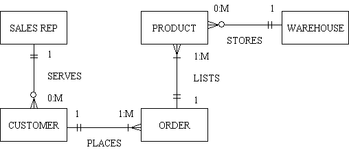
An Entity Relationship Diagram (ERD) is a data modeling technique that creates a graphical representation of the entities, and the relationships between entities, within an information system. Any ER diagram has an equivalent relational table, and any relational table has an equivalent ER diagram. ER diagramming is an invaluable aid to engineers in the design, optimization, and debugging of database programs.

• The entity is a person, object, place or event for which data is collected. It is equivalent to a database table. An entity can be defined by means of its properties, called attributes. For example, the CUSTOMER entity may have attributes for such things as name, address and telephone number.
• The relationship is the interaction between the entities. It can be described using a verb such as:
  • A customer places an order.
  • A sales rep serves a customer.
  • A order contains a product.
  • A warehouse stores a product.

In an entity-relationship diagram entities are rendered as rectangles, and relationships are portrayed as lines connecting the rectangles. One way of indicating which is the 'one' or 'parent' and which is the 'many' or 'child' in the relationship is to use an arrowhead, as in figure 4.

Figure 4 - One-to-Many relationship using arrowhead notation

This can produce an ERD as shown in figure 5:

Figure 5 - ERD with arrowhead notation

Another method is to replace the arrowhead with a crowsfoot, as shown in figure 6:

Figure 6 - One-to-Many relationship using crowsfoot notation

The relating line can be enhanced to indicate cardinality which defines the relationship between the entities in terms of numbers. An entity may be optional (zero or more) or it may be mandatory (one or more).

• A single bar indicates one.
• A double bar indicates one and only one.
• A circle indicates zero.
• A crowsfoot or arrowhead indicates many.

As well as using lines and circles the cardinality can be expressed using numbers, as in:

• One-to-One expressed as 1:1
• Zero-to-Many expressed as 0:M
• One-to-Many expressed as 1:M
• Many-to-Many expressed as N:M

This can produce an ERD as shown in figure 7:

Figure 7 - ERD with crowsfoot notation and cardinality

In plain language the relationships can be expressed as follows:

• 1 instance of a SALES REP serves 1 to many CUSTOMERS
• 1 instance of a CUSTOMER places 1 to many ORDERS
• 1 instance of an ORDER lists 1 to many PRODUCTS
• 1 instance of a WAREHOUSE stores 0 to many PRODUCTS

In order to determine if a particular design is correct here is a simple test that I use:

1. Take the written rules and construct a diagram.
2. Take the diagram and try to reconstruct the written rules.

If the output from step (2) is not the same as the input to step (1) then something is wrong. If the model allows a situation to exist which is not allowed in the real world then this could lead to serious problems. The model must be an accurate representation of the real world in order to be effective. If any ambiguities are allowed to creep in they could have disastrous consequences.

We have now completed the logical data model, but before we can construct the physical database there are several steps that must take place:

• Assign attributes (properties or values) to all the entities. After all, a table without any columns will be of little use to anyone.
• Refine the model using a process known as 'normalisation'. This ensures that each attribute is in the right place. During this process it may be necessary to create new tables and new relationships.

Data Normalisation

Relational database theory, and the principles of normalisation, were first constructed by people with a strong mathematical background. They wrote about databases using terminology which was not easily understood outside those mathematical circles. Below is an attempt to provide understandable explanations.

Data normalisation is a set of rules and techniques concerned with:

• Identifying relationships among attributes.
• Combining attributes to form relations.
• Combining relations to form a database.

It follows a set of rules worked out by E F Codd in 1970. A normalised relational database provides several benefits:

• Elimination of redundant data storage.
• Close modeling of real world entities, processes, and their relationships.
• Structuring of data so that the model is flexible.

Because the principles of normalisation were first written using the same terminology as was used to define the relational data model this led some people to think that normalisation is difficult. Nothing could be more untrue. The principles of normalisation are simple, common sense ideas that are easy to apply.

Although there are numerous steps in the normalisation process - 1NF, 2NF, 3NF, BCNF, 4NF, 5NF and DKNF - a lot of database designers often find it unnecessary to go beyond 3rd Normal Form. This does not mean that those higher forms are unimportant, just that the circumstances for which they were designed often do not exist within a particular database. However, all database designers should be aware of all the forms of normalisation so that they may be in a better position to detect when a particular rule of normalisation is broken and then decide if it is necessary to take appropriate action.

The guidelines for developing relations in 3rd Normal Form can be summarised as follows:

1st Normal Form

A table is in first normal form if all the key attributes have been defined and it contains no repeating groups.

Taking the ORDER entity in figure 7 as an example we could end up with a set of attributes like this:

This structure creates the following problems:

• Order 123 has no room for more than 3 products.
• Order 456 has wasted space for product2 and product3.

In order to create a table that is in first normal form we must extract the repeating groups and place them in a separate table, which I shall call ORDER_LINE.

I have removed 'product1', 'product2' and 'product3', so there are no repeating groups.

Each row contains one product for one order, so this allows an order to contain any number of products.

This results in a new version of the ERD, as shown in figure 8:

Figure 8 - ERD with ORDER and ORDER_LINE

The new relationships can be expressed as follows:

• 1 instance of an ORDER has 1 to many ORDER LINES
• 1 instance of a PRODUCT has 0 to many ORDER LINES

2nd Normal Form

A table is in second normal form (2NF) if and only if it is in 1NF and every non key attribute is fully functionally dependent on the whole of the primary key (i.e. there are no partial dependencies).

1. Anomalies can occur when attributes are dependent on only part of a multi-attribute (composite) key.
2. A relation is in second normal form when all non-key attributes are dependent on the whole key. That is, no attribute is dependent on only a part of the key.
3. Any relation having a key with a single attribute is in second normal form.

Take the following table structure as an example:

order(order_id, cust, cust_address, cust_contact, order_date, order_total)

Here we should realise that cust_address and cust_contact are functionally dependent on cust but not on order_id, therefore they are not dependent on the whole key. To make this table 2NF these attributes must be removed and placed somewhere else.

3rd Normal Form

A table is in third normal form (3NF) if and only if it is in 2NF and every non key attribute is non transitively dependent on the primary key (i.e. there are no transitive dependencies).

1. Anomalies can occur when a relation contains one or more transitive dependencies.
2. A relation is in 3NF when it is in 2NF and has no transitive dependencies.
3. A relation is in 3NF when 'All non-key attributes are dependent on the key, the whole key and nothing but the key'.

Take the following table structure as an example:

order(order_id, cust, cust_address, cust_contact, order_date, order_total)

Here we should realise that cust_address and cust_contact are functionally dependent on cust which is not a key. To make this table 3NF these attributes must be removed and placed somewhere else.

You must also note the use of calculated or derived fields. Take the example where a table contains PRICE, QUANTITY and EXTENDED_PRICE where EXTENDED_PRICE is calculated as QUANTITY multiplied by PRICE. As one of these values can be calculated from the other two then it need not be held in the database table. Do not assume that it is safe to drop any one of the three fields as a difference in the number of decimal places between the various fields could lead to different results due to rounding errors. For example, take the following fields:

• AMOUNT - a monetary value in home currency, to 2 decimal places.
• EXCH_RATE - exchange rate, to 9 decimal places.
• CURRENCY_AMOUNT - amount expressed in foreign currency, calculated as AMOUNT multiplied by EXCH_RATE.

If you were to drop EXCH_RATE could it be calculated back to its original 9 decimal places?

Reaching 3NF is is adequate for most practical needs, but there may be circumstances which would benefit from further normalisation.

Boyce-Codd Normal Form

A table is in Boyce-Codd normal form (BCNF) if and only if it is in 3NF and every determinant is a candidate key.

1. Anomalies can occur in relations in 3NF if there is a composite key in which part of that key has a determinant which is not itself a candidate key.
2. This can be expressed as R(A,B,C), CA where:
   • The relation contains attributes A, B and C.
   • A and B form a candidate key.
   • C is the determinant for A (A is functionally dependent on C).
   • C is not part of any key.
3. Anomalies can also occur where a relation contains several candidate keys where:
   • The keys contain more than one attribute (they are composite keys).
   • An attribute is common to more than one key.

Take the following table structure as an example:

schedule(campus, course, class, time, room/bldg)

Take the following sample data:

Note that no two buildings on any of the university campuses have the same name, thus ROOM/BLDGCAMPUS. As the determinant is not a candidate key this table is NOT in Boyce-Codd normal form.

This table should be decomposed into the following relations:

R1(course, class, room/bldg, time)

R2(room/bldg, campus)

As another example take the following structure:

enrol(student#, s_name, course#, c_name, date_enrolled)

This table has the following candidate keys:

• (student#, course#)
• (student#, c_name)
• (s_name, course#) - this assumes that s_name is a unique identifier
• (s_name, c_name) - this assumes that c_name is a unique identifier

The relation is in 3NF but not in BCNF because of the following dependencies:

• student#s_name
• course#c_name

4th Normal Form

A table is in fourth normal form (4NF) if and only if it is in BCNF and contains no more than one multi-valued dependency.

1. Anomalies can occur in relations in BCNF if there is more than one multi-valued dependency.
2. If AB and AC but B and C are unrelated, ie A(B,C) is false, then we have more than one multi-valued dependency.
3. A relation is in 4NF when it is in BCNF and has no more than one multi-valued dependency.

Take the following table structure as an example:

info(employee#, skills, hobbies)

Take the following sample data:

This table is difficult to maintain since adding a new hobby requires multiple new rows corresponding to each skill. This problem is created by the pair of multi-valued dependencies EMPLOYEE#SKILLS and EMPLOYEE#HOBBIES. A much better alternative would be to decompose INFO into two relations:

skills(employee#, skill)

hobbies(employee#, hobby)

5th (Projection-Join) Normal Form

A table is in fifth normal form (5NF) or Projection-Join Normal Form (PJNF) if it is in 4NF and it cannot have a lossless decomposition into any number of smaller tables.

Another way of expressing this is:

... and each join dependency is a consequence of the candidate keys.

Yet another way of expressing this is:

... and there are no pairwise cyclical dependencies in the primary key comprised of three or more attributes.

• Anomalies can occur in relations in 4NF if the primary key has three or more fields.
• 5NF is based on the concept of join dependence - if a relation cannot be decomposed any further then it is in 5NF.
• Pairwise cyclical dependency means that:
  • You always need to know two values (pairwise).
  • For any one you must know the other two (cyclical).

Take the following table structure as an example:

buying(buyer, vendor, item)

This is used to track buyers, what they buy, and from whom they buy.

Take the following sample data:

The question is, what do you do if Claiborne starts to sell Jeans? How many records must you create to record this fact?

The problem is there are pairwise cyclical dependencies in the primary key. That is, in order to determine the item you must know the buyer and vendor, and to determine the vendor you must know the buyer and the item, and finally to know the buyer you must know the vendor and the item.

The solution is to break this one table into three tables; Buyer-Vendor, Buyer-Item, and Vendor-Item.

6th (Domain-Key) Normal Form

A table is in sixth normal form (6NF) or Domain-Key normal form (DKNF) if it is in 5NF and if all constraints and dependencies that should hold on the relation can be enforced simply by enforcing the domain constraints and the key constraints specified on the relation.

Another way of expressing this is:

... if every constraint on the table is a logical consequence of the definition of keys and domains.

1. An domain constraint (better called an attribute constraint) is simply a constraint to the effect a given attribute A of R takes its values from some given domain D.
2. A key constraint is simply a constraint to the effect that a given set A, B, ..., C of R constitutes a key for R.

This standard was proposed by Ron Fagin in 1981, but interestingly enough he made no note of multi-valued dependencies, join dependencies, or functional dependencies in his paper and did not demonstrate how to achieve DKNF. However, he did manage to demonstrate that DKNF is often impossible to achieve.

If relation R is in DKNF, then it is sufficient to enforce the domain and key constraints for R, and all constraints on R will be enforced automatically. Enforcing those domain and key constraints is, of course, very simple (most DBMS products do it already). To be specific, enforcing domain constraints just means checking that attribute values are always values from the applicable domain (i.e., values of the right type); enforcing key constraints just means checking that key values are unique.

Unfortunately lots of relations are not in DKNF in the first place. For example, suppose there's a constraint on R to the effect that R must contain at least ten tuples. Then that constraint is certainly not a consequence of the domain and key constraints that apply to R, and so R is not in DKNF. The sad fact is, not all relations can be reduced to DKNF; nor do we know the answer to the question "Exactly when can a relation be so reduced?"

De-Normalisation

Denormalisation is the process of modifying a perfectly normalised database design for performance reasons. Denormalisation is a natural and necessary part of database design, but must follow proper normalisation. Here are a few words from C J Date on denormalisation:

The general idea of normalization...is that the database designer should aim for relations in the "ultimate" normal form (5NF). However, this recommendation should not be construed as law. Sometimes there are good reasons for flouting the principles of normalization.... The only hard requirement is that relations be in at least first normal form. Indeed, this is as good a place as any to make the point that database design can be an extremely complex task.... Normalization theory is a useful aid in the process, but it is not a panacea; anyone designing a database is certainly advised to be familiar with the basic techniques of normalization...but we do not mean to suggest that the design should necessarily be based on normalization principles alone.

C.J. Date
An Introduction to Database Systems
Pages 528-529

In the 1970s and 1980s when computer hardware was bulky, expensive and slow it was often considered necessary to denormalise the data in order to achieve acceptable performance, but this performance boost often came with a cost (refer to Modification Anomalies). By comparison, computer hardware in the 21st century is extremely compact, extremely cheap and extremely fast. When this is coupled with the enhanced performance from today's DBMS engines the performance from a normalised database is often acceptable, therefore there is less need for any denormalisation.

However, under certain conditions denormalisation can be perfectly acceptable. Take the following table as an example:

This table is NOT in 3rd normal form because the city and state are dependent upon the ZIP code. To place this table in 3NF, two separate tables would be created - one containing the company name and ZIP code and the other containing city, state, ZIP code pairings.

This may seem overly complex for daily applications and indeed it may be. Database designers should always keep in mind the tradeoffs between higher level normal forms and the resource issues that complexity creates.

Deliberate denormalisation is commonplace when you're optimizing performance. If you continuously draw data from a related table, it may make sense to duplicate the data redundantly. Denormalisation always makes your system potentially less efficient and flexible, so denormalise as needed, but not frivolously.

There are techniques for improving performance that involve storing redundant or calculated data. Some of these techniques break the rules of normalisation, others do not. Sometimes real world requirements justify breaking the rules. Intelligently and consciously breaking the rules of normalisation for performance purposes is an accepted practice, and should only be done when the benefits of the change justify breaking the rule.

Compound Fields

A compound field is a field whose value is the combination of two or more fields in the same record. The cost of using compound fields is the space they occupy and the code needed to maintain them. (Compound fields typically violate 2NF or 3NF.)

For example, if your database has a table with addresses including city and state, you can create a compound field (call it City_State) that is made up of the concatenation of the city and state fields. Sorts and queries on City_State are much faster than the same sort or query using the two source fields - sometimes even 40 times faster.

The downside of compound fields for the developer is that you have to write code to make sure that the City_State field is updated whenever either the city or the state field value changes. This is not difficult to do, but it is important that there are no 'leaks', or situations where the source data changes and, through some oversight, the compound field value is not updated.

Summary Fields

A summary field is a field in a one table record whose value is based on data in related-many table records. Summary fields eliminate repetitive and time-consuming cross-table calculations and make calculated results directly available for end-user queries, sorts, and reports without new programming. One-table fields that summarise values in multiple related records are a powerful optimization tool. Imagine tracking invoices without maintaining the invoice total! Summary fields like this do not violate the rules of normalisation. Normalisation is often misconceived as forbidding the storage of calculated values, leading people to avoid appropriate summary fields.

There are two costs to consider when contemplating using a summary field: the coding time required to maintain accurate data and the space required to store the summary field.

Some typical summary fields which you may encounter in an accounting system are:

• For an INVOICE the invoice amount is the total of the amounts on all INVOICE_LINE records for that invoice.
• For an ACCOUNT the account balance will be the sum total of the amounts on all INVOICE and PAYMENT records for that account.

Summary Tables

A summary table is a table whose records summarise large amounts of related data or the results of a series of calculations. The entire table is maintained to optimise reporting, querying, and generating cross-table selections. Summary tables contain derived data from multiple records and do not necessarily violate the rules of normalisation. People often overlook summary tables based on the misconception that derived data is necessarily denormalised.

In order for a summary table to be useful it needs to be accurate. This means you need to update summary records whenever source records change. This task can be taken care of in the program code, or in a database trigger (preferred), or in a batch process. You must also make sure to update summary records if you change source data in your code. Keeping the data valid requires extra work and introduces the possibility of coding errors, so you should factor this cost in when deciding if you are going to use this technique.

Optional Attributes that exist as a group

As mentioned in the guidelines for developing relations in 3rd normal form all relations which share the same primary key are supposed to be combined into the same table. However, there are circumstances where is is perfectly valid to ignore this rule. Take the following example which I encountered in 1984:

• A finance company gives loans to customers, and a record is kept of each customer's repayments.
• If a customer does not meet a scheduled repayment then his account goes into arrears and special action needs to be taken.
• Of the total customer base about 5% are in arrears at any one time.

This means that with 100,000 customers there will be roughly 5,000 in arrears. If the arrears data is held on the same record as the basic customer data (both sets of data have customer_id as the primary key) then it requires searching through all 100,000 records to locate those which are in arrears. This is not very efficient. One method tried was to create an index on account_status which identified whether the account was in arrears or not, but the improvement (due to the speed of the hardware and the limitations of the database engine) was minimal.

A solution in these circumstances is to extract all the attributes which deal with arrears and put them in a separate table. Thus if there are 5,000 customers in arrears you can reference a table which contains only 5,000 records. As the arrears data is subordinate to the customer data the arrears table must be the 'child' in the relationship with the customer 'parent'. It would be possible to give the arrears table a different primary key as well as the foreign key to the customer table, but this would allow the customerarrears relationship to be one-to-many instead of one-to-one. To enforce this constraint the foreign key and the primary key should be exactly the same.

This situation can be expressed using the following structure:

R (K, A, B, C, X, Y, Z) where:

1. Attribute K is the primary key.
2. Attributes (A B C) exist all the time.
3. Attributes (X Y Z) exist some of the time (but always as a group under the same circumstances).
4. Attributes (X Y Z) require special processing.

After denormalising the result is two separate relations, as follows:

• R1 (K, A, B, C)
• R2 (K, X, Y, Z) where K is also the foreign key to R1

Personal Guidelines

Even if you obey all the preceding rules it is still possible to produce a database design that causes problems during development. I have come across many different implementation tips and techniques over the years, and some that have worked in one database system have been successfully carried forward into a new database system. Some tips, on the other hand, may only be applicable to a particular database system.

For particular options and limitations you must refer to your database manual.

Database Names

1. Database names should be short and meaningful, such as products, purchasing and sales.
   • Short, but not too short, as in prod or purch.
   • Meaningful but not verbose, as in 'the database used to store product details'.
2. Do not waste time using a prefix such as db to identify database names. The SQL syntax analyser has the intelligence to work that out for itself - so should you.
3. If your DBMS allows a mixture of upper and lowercase names, and it is case sensitive, it is better to stick to a standard naming convention such as:
   • All uppercase.
   • All lowercase (my preference - see The choice between upper and lower case).
   • Leading uppercase, remainder lowercase.
   Inconsistencies may lead to confusion, confusion may lead to mistakes, mistakes can lead to disasters.
4. If a database name contains more than one word, such as in sales orders and purchase orders, decide how to deal with it:
   • Separate the words with a single space, as in sales orders (note that some DBMSs do not allow embedded spaces, while most languages will require such names to be enclosed in quotes).
   • Separate the words with an underscore, as in sales_orders (my preference - see The choice between upper and lower case).
   • Separate the words with a hyphen, as in sales-orders.
   • Use camel caps, as in SalesOrders.
   Again, be consistent.
5. Rather than putting all the tables into a single database it may be better to create separate databases for each logically related set of tables. This may help with security, archiving, replication, etc.

Table Names

1. Table names should be short and meaningful, such as part, customer and invoice.
   • Short, but not too short.
   • Meaningful, but not verbose.
2. Do not waste time using a prefix such as tbl to identify table names. The SQL syntax analyser has the intelligence to work that out for itself - so should you.
3. Table names should be in the singular (e.g. customer not customers). The fact that a table may contain multiple entries is irrelevant - any multiplicity can be derived from the existence of one-to-many relationships.
4. If your DBMS allows a mixture of upper and lowercase names, and it is case sensitive, It is better to stick to a standard naming convention such as:
   • All uppercase.
   • All lowercase. (my preference - see The choice between upper and lower case)
   • Leading uppercase, remainder lowercase.
   Inconsistencies may lead to confusion, confusion may lead to mistakes, mistakes can lead to disasters.
5. If a table name contains more than one word, such as in sales order and purchase order, decide how to deal with it:
   • Separate the words with a single space, as in sales order (note that some DBMSs do not allow embedded spaces, while most languages will require such names to be enclosed in quotes).
   • Separate the words with an underscore, as in sales_order (my preference - see The choice between upper and lower case).
   • Separate the words with a hyphen, as in sales-order.
   • Use camel caps, as in SalesOrder.
   Again, be consistent.
6. Be careful if the same table name is used in more than one database - it may lead to confusion.

Field Names

1. Field names should be short and meaningful, such as part_name and customer_name.
   • Short, but not too short, such as in ptnam.
   • Meaningful, but not verbose, such as the name of the part.
2. Do not waste time using a prefix such as col or fld to identify column/field names. The SQL syntax analyser has the intelligence to work that out for itself - so should you.
3. If your DBMS allows a mixture of upper and lowercase names, and it is case sensitive, it is better to stick to a standard naming convention such as:
   • All uppercase.
   • All lowercase. (my preference - see The choice between upper and lower case)
   • Leading uppercase, remainder lowercase.
   Inconsistencies may lead to confusion, confusion may lead to mistakes, mistakes can lead to disasters.
4. If a field name contains more than one word, such as in part name and customer name, decide how to deal with it:
   • Separate the words with a single space, as in part name (note that some DBMSs do not allow embedded spaces, while most languages will require such names to be enclosed in quotes).
   • Separate the words with an underscore, as in part_name (my preference - see The choice between upper and lower case).
   • Separate the words with a hyphen, as in part-name.
   • Use camel caps, as in PartName.
   Again, be consistent.
5. Common words in field names may be abbreviated, but be consistent.
   • Do not allow a mixture of abbreviations, such as 'no', 'num' and 'nbr' for 'number'.
   • Publish a list of standard abbreviations and enforce it.
6. Although field names must be unique within a table, it is possible to use the same name on multiple tables even if they are unrelated, or they do not share the same set of possible values. It is recommended that this practice should be avoided, for reasons described in Field names should identify their content and The naming of Foreign Keys.

Primary Keys

1. It is recommended that the primary key of an entity should be constructed from the table name with a suffix of _ID. This makes it easy to identify the primary key in a long list of field names.
2. Do not waste time using a prefix such as pk to identify primary key fields. This has absolutely no meaning to any database engine or any application.
3. Avoid using generic names for all primary keys. It may seem a clever idea to use the name ID for every primary key field, but this causes problems:
   • It causes the same name to appear on multiple tables with totally different contexts. The string ID='ABC123' is extremely vague as it gives no idea of the entity being referenced. Is it an invoice id, customer id, or what?
   • It also causes a problem with foreign keys.
4. There is no rule that says a primary key must consist of a single attribute - both simple and composite keys are allowed - so don't waste time creating artificial keys.
5. Avoid the unnecessary use of technical keys. If a table already contains a satisfactory unique identifier, whether composite or simple, there is no need to create another one. Although the use of a technical key can be justified in certain circumstances, it takes intelligence to know when those circumstances are right. The indiscriminate use of technical keys shows a distinct lack of intelligence. For further views on this subject please refer to Technical Keys - Their Uses and Abuses.

Foreign Keys

1. It is recommended that where a foreign key is required that you use the same name as that of the associated primary key on the foreign table. It is a requirement of a relational join that two relations can only be joined when they share at least one common attribute, and this should be taken to mean the attribute name(s) as well as the value(s). Thus where the customer and invoice tables are joined in a parent-child relationship the following will result:
   • The primary key of customer will be customer_id.
   • The primary key of invoice will be invoice_id.
   • The foreign key which joins invoice to customer will be customer_id.
2. For MySQL users this means that the shortened version of the join condition may be used:
   • Short: A LEFT JOIN B USING (a,b,c)
   • Long: A LEFT JOIN B ON (A.a=B.a AND A.b=B.b AND A.c=B.c)
3. The only exception to this naming recommendation should be where a table contains more than one foreign key to the same parent table, in which case the names must be changed to avoid duplicates. In this situation I would simply add a meaningful suffix to each name to identify the usage, such as:
   • To signify movement I would use location_id_from and location_id_to.
   • To signify positions in a hierarchy I would use node_id_snr and node_id_jnr.
   • To signify replacement I would use part_id_old and part_id_new.
   • In some cases different names can be used provided that they are recognisable, so that you can use employer_id and employee_id instead of person_id_snr and person_id_jnr.
   I prefer to use a suffix rather than a prefix as it makes the leading characters match (as in PART_ID_old and PART_ID_new) instead of having the trailing characters match (as in old_PART_ID and new_PART_ID).
4. Do not waste time using a prefix such as fk to identify foreign key fields. This has absolutely no meaning to any database engine or any application.

Note that a foreign key is not the same as a foreign key constraint. Refer to Referential Integrity for more details.

Generating Unique ids

Where a technical primary key is used a mechanism is required that will generate new and unique values. Such keys are usually numeric, so there are several methods available:

1. Some database engines will maintain a set of sequence numbers for you which can be referenced using code such as :

   SELECT <seq_name>.NEXTVAL FROM DUAL
   

   Using such a sequence is a two-step procedure:
   • Access the sequence to obtain a value.
   • Use the supplied value on an INSERT statement.

   It is sometimes possible to access the sequence directly from an INSERT statement, as in the following:

   INSERT INTO tablename (col1,col2,...) VALUES (tablename_seq.nextval,'value2',...)
   

   If the number just used needs to be retrieved so that it can be passed back to the application it can be done so with the following:

   SELECT <seq_name>.CURRVAL FROM DUAL
   

   I have used this method, but a disadvantage that I have found is that the DBMS has no knowledge of what primary key is linked to which sequence, so it is possible to insert a record with a key not obtained from the sequence and thus cause the two to become unsynchronised. The next time the sequence is used it could therefore generate a value which already exists as a key and therefore cause an INSERT error.

2. Some database engines will allow you to specify a numeric field as 'auto-increment', and on an INSERT they will automatically generate the next available number (provided that no value is provided for that field in the first place). This is better than the previous method because:
   • The sequence is tied directly to a particular database table and is not a separate object, thus it is impossible to become unsynchronised.
   • It is not necessary to access the sequence then use the returned value on an INSERT statement - just leave the field empty and the DBMS will fill in the value automatically.
3. While the previous methods have their merits, they both have a common failing in that they are not-standard extensions to the SQL standard, therefore they are not available in all SQL-compliant database engines. This becomes an important factor if it is ever decided to switch to another database engine. A truly portable method which uses a standard technique and can therefore be used in any SQL-compliant database is to use an SQL statement similar to the following to obtain a unique key for a table:

   SELECT max(table_id) FROM <tablename>
   table_id = table_id+1
   

   Some people seem to think that this method is inefficient as it requires a full table search, but they are missing the fact that table_id is a primary key, therefore the values are held within an index. The SELECT max(...) statement will automatically be optimised to go straight to the last value in the index, therefore the result is obtained with almost no overhead. This would not be the case if I used SELECT count(...) as this would have to physically count the number of entries. Another reason for not using SELECT count(...) is that if records were to be deleted then record count would be out of step with the highest current value.
4. The Radicore development framework has separate data access objects for each DBMS to which it can connect. This means that the different code for dealing with auto_increment keys can be contained within each object, so is totally transparent to the application. All that is necessary is that the key be identified as 'auto_increment' in the Data Dictionary and the database object will take care of all the necessary processing.

Criticisms

Some people disagree with my ideas, but usually because they have limited experience and only know what they have been taught. What I have stated here is the result of decades of experience using various database systems with various languages. This is what I have learned, and goes beyond what I have been taught. There are valid reasons for some of the preferences I have stated in this document, and it may prove beneficial to state these in more detail.

The choice between upper and lower case

When I first started programming in the 1970s all coding was input via punched cards, not a VDU (that's a Visual Display Unit to the uninitiated), and there was no such thing as lowercase as the computer, a UNIVAC mainframe, used a 6-bit character instead of an 8-bit byte and did not have enough room to deal with both lower and uppercase characters. CONSEQUENTLY EVERYTHING HAD TO BE IN UPPER CASE. When I progressed to a system where both cases were possible neither the operating system nor the programming language cared which was used - they were both case-insensitive. By common consent all the programmers preferred to use lowercase for everything. The use of uppercase was considered TO BE THE EQUIVALENT OF SHOUTING and was discouraged, except where something important needed to stand out.

Until the last few years all the operating systems, database systems, programming languages and text editors have been case-insensitive. The UNIX operating system and its derivatives are case-sensitive (for God's sake WHY??). The PHP programming language is case-sensitive in certain areas.

I do not like systems which are case-sensitive for the following reasons:

• I have been working for 30 years with systems which have been case-insensitive and I see no justification in making the switch.
• Case does not make a difference in any spoken language, so why should it make a difference in any computer language?
• When I am merrily hammering away at the keyboard I do not like all those pauses where I have to reach for the shift key. It tends to interrupt my train of thought, and I do not like to be interrupted with trivialities.
• To my knowledge there is no database system which is case-sensitive, so when I am writing code to access a database I do not like to be told which case to use. If the SQL language does not care what case is used when referring to database, table and column names, then what is the justification for turning it into an issue?
• With the growing trend of being able to speak to a computer instead of using a keyboard, how frustrating will it become if you have to specify that particular words and letters are in upper or lower case?

That is why my preference is for all database, table and field names to be in lowercase as it works the same for both case-sensitive and case-insensitive systems, so I don't get suddenly caught out when the software decides to get picky. This also means that I use underscore separators instead of those ugly CamelCaps (i.e. 'field_name' instead of 'FieldName').

This topic is discussed in more detail in Case Sensitive Software is EVIL.

The use of unique and non-unique field names

Some people think that my habit of including the table name inside a field name (as in CUSTOMER.CUSTOMER_ID instead of their preferred CUSTOMER.ID) introduces a level of redundancy and is therefore wrong. I consider this view to be too narrow as it does not cater for all the different circumstances I have encountered over the years. This becomes most apparent when you construct an SQL query with lots of JOINs to foreign tables which all have a primary key field called ID. The result set returned by the query is an associative array of name=value pairs in which each column name is never qualified with its table name. If this result set contains several fields with the name "ID" then guess what? Only the last one will actually be present as all previous fields with the same name will be overwritten. The only way around this is to give each field an alias in the SELECT portion of the query, as in customer.id AS customer_id so that each field in the result is given a unique name so that it will not be overwritten if that name appears in another table. So by saving keystrokes at the DDL stage you end up by using more keystrokes at the DML stage. So not much of a saving after all.

Field names should identify their content

Over many years I have come to adopt a fairly straightforward convention with the naming of fields:

• Field names should give some idea of their content.

  If I see several tables which all contain field names such as ID and DESCRIPTION it makes me want to reach for the rubber gloves, disinfectant and scrubbing brush. A field named ID simply says that it contains an identity, but the identity of what? A field named DESCRIPTION simply says that it contains a description, but the description of what?

  One of the first database systems which I used did not allow field definitions to be included within the table definitions inside the schema. Instead all the fields were defined in one area, and the table definitions simply listed the fields which they contained. This meant that a field was defined with one set of attributes (type and size) and those attributes could not be changed at the table level. Thus ID could not be C10 in one table and C30 in another. The only time we had fields with the same name existing on more than one table was where there was a logical relationship between records which had the same values in those fields.

  Because of this it became standard practice to have unique field names on each table using the table name as a prefix, such as table_id and table_desc. One of the benefits of this approach was that we could build standard code which provided the correct label and help text based on nothing more than the field name itself.

  When performing sql JOINS between tables which have common field names that are unrelated you have to give each field a unique alias name before you can access its content. If each of these fields were given a unique name to begin with then this step would not be necessary.

• Fields with the same context should have the same name.

  If primary keys are named table_id instead of just id it then becomes possible, when naming foreign key fields on related tables, to use the same name for both the primary key and the foreign key. This makes it easier for a human being to recognise certain fields for what they are - anything ending in _id is a key field, and if the table prefix is not the current table then it is a foreign key to that table. This is what we called "self-documenting field names".

  In some circumstances it may not be possible to use the same name. This happens when the same field needs to appear more than once in the same table. In this case I would start with the same basic name and add a suffix for further identification, such as having location_id_FROM and location_id_TO to identify movements from one location to another, or having node_id_SNR and node_id_JNR to identify the senior and junior nodes in a hierarchical relationship.

• Fields with different context should have different names.

  It is not just primary key fields which should have unique names instead of sharing the common name of id. Non-key fields should follow the same convention for the same reasons. For example, if the CUSTOMER table has a STATUS field with one set of values and the INVOICE table has a STATUS field with another set of values then you should resist the temptation to give the two different fields the same common name of STATUS. They should be given proper names such as CUST_STATUS and INV_STATUS. They are different fields with different meanings, therefore they deserve to have different names.

  The breaking of this simple rule cased problems in one of the short-lived new-fangled languages that I used many years ago. This tool was built on the assumption that fields with the same name that existed on more than one table implied a relationship between those tables. If you tried to perform a join between two tables this software would look for field names which existed on both tables and automatically perform a natural join using those fields. This caused our programs not to find the right records when we performed a join, and the only way we could fix it was to give different names to unrelated fields.

Those conventions arose out of experience, to avoid certain problems which were encountered with certain languages. Every time I see these conventions broken I do not have to wait long before I see the same problems reappearing.

The naming of Foreign Keys

In any relationship the foreign key field(s) on the child/junior table are linked with the primary key field(s) on the parent/senior table. These related fields do not have to have the same name as it is still possible to perform a join, as shown in the following example:

SELECT field1, field2, field3
   FROM first_table
   LEFT [OUTER] JOIN second_table
   ON (first_table.keyfield = second_table.foreign_keyfield)

However, if the fields have the same name then it is possible to replace the ON expression with a shorter USING expression, as in the following example:

SELECT field1, field2, field3
   FROM first_table
   LEFT [OUTER] JOIN second_table
   USING (field1)

This feature is available in popular databases such as MySQL, PostgreSQL and Oracle, so it just goes to show that using identical field names is a recognised practice that has its benefits.

Not only does the use of identical names have an advantage when performing joins in an SQL query, it also has advantages when simulating joins in your software. By this I mean where the reading of the two tables is performed in separate operations. It is possible to perform this using standard code with the following logic:

• Operation (1) perform the following after each database row has been read:
  • Identify the field(s) which constitute the primary key for the first table.
  • Extract the values for those fields from the current row.
  • Construct a string in the format field1='value1' [field2='value2'].
  • Pass this string to the next operation.
• Operation (2) performs the following:
  • Use the string passed down from the previous operation as the WHERE clause in a SELECT statement.
  • Execute the query on the second table.
  • Return the result back to the previous operation.

It is possible to perform these functions using standard code that never has to be customised for any particular database table. I should know as I have done it in two completely different languages. The only time that manual intervention (i.e. extra code) is required is where the field names are not exactly the same, which forces operation (2) to convert primary_key_field='value' to foreign_key_field='value' before it can execute the query. Experienced programmers should instantly recognise that the need for extra code incurs its own overhead:

• The time taken to actually write this extra code.
• The time taken to test that the right code has been put in the right place.
• The time taken to amend this code should there be any database changes in the future.

The only occasion where fields with the same name are not possible is when a table contains multiple versions of that field. This is where I would add a suffix to give some extra meaning. For example:

• In a table which records movements or ranges I would have <table>_ID_FROM and <table>_ID_TO.
• In a table which records a senior-to-junior hierarchy I would have <table>_ID_SNR and <table>_ID_JNR.

My view of field names can be summed up as follows:

• Fields with the same context should have the same name.
• Fields with different context should have different names.
• Key fields, whether primary or foreign, should be in the format <table>_id.
• Duplicate foreign keys should be in the format <table>_id_<suffix>

References

• Technical Keys - Their Uses and Abuses by Tony Marston
• Database Design - are you Novice, Ninja or Nincompoop? by Tony Marston
• How to handle a Many-to-Many relationship with PHP and MySQL by Tony Marston

• Rules of Data Normalization from DataModel.org
• Choosing a Primary Key: Natural or Surrogate? by Scott Wambler
• Surrogate Keys: Part 1, Best Practice or Wrong-Headed Dogma? from the Actian Community Blogs
• Surrogate Keys: Part 2, The Boring Bit from the Actian Community Blogs
• Surrogate Keys: Part 3, Surrogates for Composites from the Actian Community Blogs
• Surrogate Keys: Part 4, In Search of a Niche from the Actian Community Blogs
• Surrogate Keys: Part 5, Pitfalls, Booby-Traps and the 1970s Resurrected from the Actian Community Blogs
• Database Design from wikipedia.org
• Normalisation from wikipedia.org
• Composite Primary Keys from Jeff's SQL Server Blog
• Distinguishing data from code from Jeff's SQL Server Blog
• Data belongs in your tables -- not in your code from Jeff's SQL Server Blog
• SQL Data Modeling: Entities versus Attributes from Jeff's SQL Server Blog
• Don't Let Output Dictate your Database Design from Jeff's SQL Server Blog

Amendment History